Data Lab 2 - Navigating RStudio: Using R Scripts and R Markdown Files

Navigating RStudio

In this tutorial, we’ll learn how to write R code using an R Script and using an R Markdown document. You can think of an R Script as a file where you store your R commands so that you don’t have to manually type each command into the Console’s command line (this would get really confusing for large projects!). You can think of an R Markdown document as a combination text editor (like Microsoft Word) and R Script. We’ll see that using an R Markdown document can be a good way to organize our R code and the output that code generates.

We’ll work through this tutorial in class using the examples in ModernDive Chapter 1 and you’ll create additional R Markdown documents for other tutorials and homework assignments throughout the semester.

Open a new R Project

Navigate to the File -> New Project tab in RStudio. Select “New Directory” to create a new folder specific to this project. Since we’re going to be working with multiple projects throughout the course, it might be helpful to create a master directory for HPAM7660 and then subfolders for individual Data Lab projects. Next choose “New Project” from the Project Type menu, select the master directory you just created, name the subfolder (let’s call it “Data Lab 2”), and press the “Create Project” button.

RStudio Window

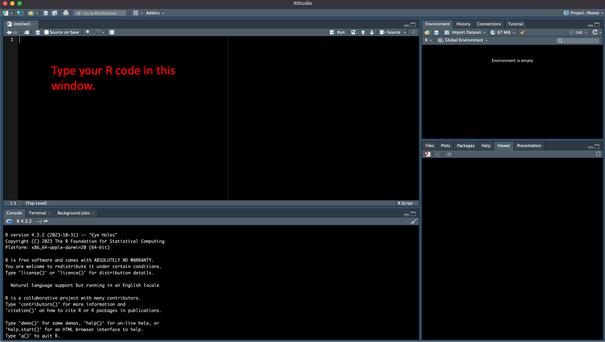
Let’s take a minute to briefly go over the RStudio interface. When you open RStudio, you’ll typically see the following three windows.

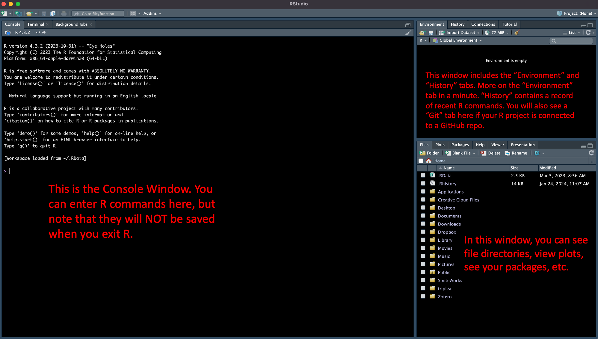
There’s a lot more here, but we’ll cover other aspects of RStudio as they come up in our tutorials and problem sets.

Console Command Line

Now that we have created a new R project , let’s start by running a few commands in the RStudio Console Window command line. This is the window at the bottom of RStudio (make sure the “Console” tab is selected). Throughout this tutorial, we’ll be working through the examples in Chapter 1.4 of ModernDive.

First we need to install and load the packages we’ll need for the tutorial (you may already have some of these packages installed, but it won’t hurt to reinstall them). Type each of the following commands in to the RStudio command line:

install.packages("nycflights13")
install.packages("dplyr")
install.packages("knitr")

library(nycflights13)
library(dplyr)
library(knitr)

Exploring Data Frames

Now that we’ve loaded the packages and libraries, let’s take a look at the data objects contained in nycflights13. To do so, click on the drop down icon next to “Global Environment” and select “package:nycflights13”.

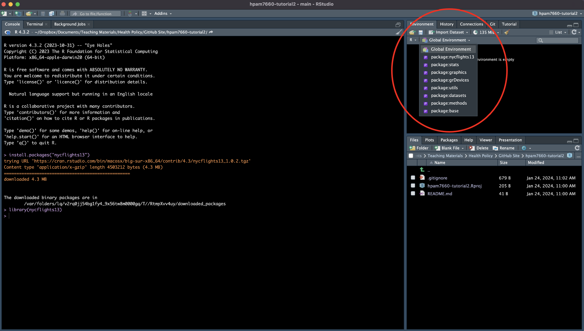
You should now see a series of objects in the “Environment” window.

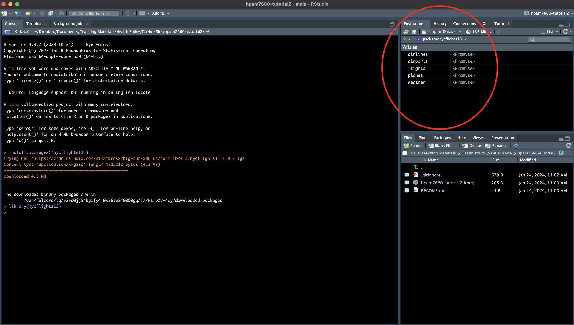
Let’s take a look at each of these objects to see what information they contain. Type the following code into the Console Window command line and hit enter:

flights

You should now see a “tibble” that displays the first 8 columns and the first 10 rows of the flights data frame. The tibble also tells us that the data frame contains 336,766 more rows (beyond those displayed in the Console Window) and 5 more variables/columns (each of which is listed).

There are several other ways that we could examine the flights data frame including:

1. Using the View() function to open RStudio’s built-in data viewer. This allows us to scroll through all columns and rows in the data frame.
2. Using the glimpse() function, which is part of the dplyr package. This is similar to the tibble that we saw by simply typing flights into the console, but also includes each variables data type (e.g., integer, double, character, etc.)
3. Using the kable() function, which is part of the knitr package. This function is helpful when we want to generate formatted output in an RMarkdown document, but it’s important to note that kable will print the entire data frame by default.

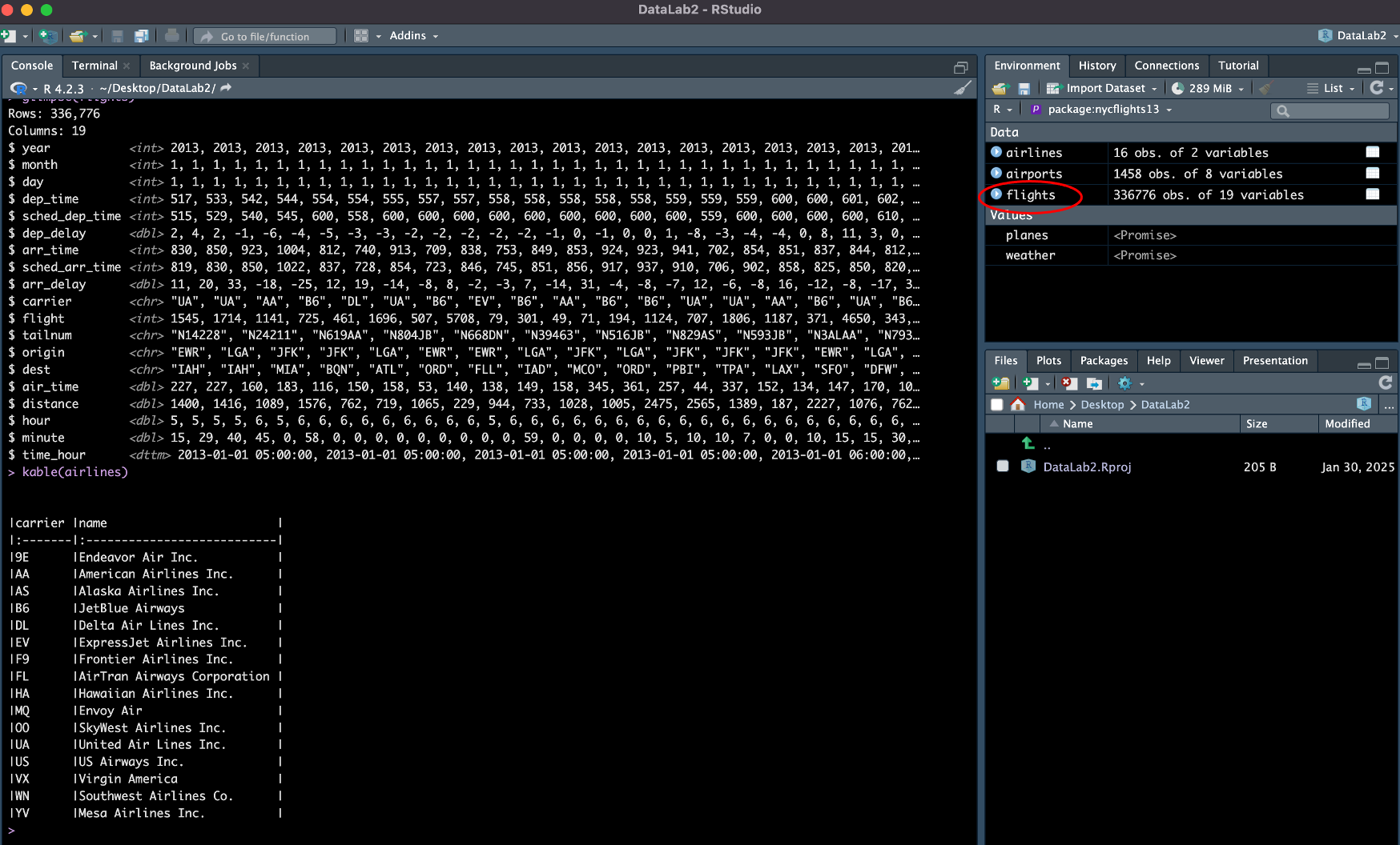
Let’s try some of these out. Use the glimpse function to take a look at the flights data frame by typing glimpse(flights) into the console command line. Next, use the kable function to examine the airlines data frame by typing kable(airlines) into the console command line.

Sometimes it’s nice to take a look at the dataset as you might see it in a .csv or Excel file layout. To do this, click on flights in the Data window:

Once you’ve had a chance to look through the data, close out the data preview window and we’ll start making some changes to the data.

Data Manipulation

Suppose we want a list of flight numbers and delay times for each United Airlines flight that was delayed by 4 hours or longer in January 2013. First, we can subset the data so that we only retain United Airlines flights. We can do this using the carrier variable since the code “UA” in this field identifies United Airlines flights. Go ahead and type the following into the Console command line and hit enter:

ua_flights <- filter(flights, carrier == "UA")

Click the drop down arrow in the Environment tab to go back to “Global Environment” and you should see new data object called “ua_flights”. Let’s take a look at it using one of the viewing methods above (use whichever you prefer).

Now we need to determine which UA flights in January 2013 were delayed by 4 hours or longer. We can do another subset of the data using the year, month, and arr_delay variables (notice that the arr_delay variable is measured in minutes). Type the following into the Console command line and hit enter:

ua_delay <- filter(ua_flights, year == 2013, month == 1, arr_delay >= 240)

Now we have a data frame that includes all UA flights that were delayed by 4 hours or longer in January 2013. Notice that we didn’t need a separate filter command for each argument (i.e., year, month, and arr_delay), we simply combined them all into a single filter command.

Finally, since we’re really only interested in the flight numbers and delay times, we can get rid of the extraneous variables in the data frame using the select command.

ua_final <- select(ua_delay, flight, arr_delay)

Now that we have our final dataframe, let’s take a look at the table of flight delays using the kable function:

kable(ua_final)

You should see a list of flight numbers and arrival delays (recorded in minutes). It looks like there were 12 flights in January 2003 that were delayed by 4 hours or longer.

Using R Scripts

So far so good, but what happens if we were to close out of RStudio? Or, say 6 months from now, we decide we want to re-generate the table we just made? Entering commands directly into the Console Window command line is not a very good way to structure our workflow because once those comments are gone, they’re gone for good! A better way to track our work and ensure that we can reproduce our results if necessary is to use an R script file to write our code. Let’s take a look.

Navigate to the File -> New File -> R Script tab in RStudio. This should open a new window in RStudio called the “Source” window and a document called “Untitled1” where you can write and save your R code.

Let’s give this file a name and then recreate our United Airlines flight delay table by writing the code we entered directly into the command line into our R Script.

To name the file you can click on the save icon in the menu bar or navigate to File -> Save. Either way, you should be prompted to name the file (which will have a .R extension) and choose a location for saving. Let’s call this file DataLab_2 and save it in the folder you created for this R project.

Now type the code below into the R script (note that I have combined a couple of lines from the previous version):

library(nycflights13)
library(dplyr)
library(knitr)

ua_delay <- filter(flights, carrier == "UA", year == 2013, month == 1, arr_delay >= 240)
ua_final <- select(ua_delay, flight, arr_delay)
kable(ua_final)

Once you’ve typed this into your R Script, save it, and click on the “Run” button in the menu bar. You should see the code run and the output table displayed in the Console window. Now if you exit RStudio, you’ll have the script file that you can run at a later date and reproduce the exact same table.

Also note that I included the library() commands in the R script, but not the install.packages() commands. You only need to install an R package one time. Once you’ve installed a package it stays installed. However, R does not automatically load those packages each session. So in order to use the packages you’ve installed, you need to tell R to load them each time you start a new session by using the library() command. It wouldn’t hurt anything to include the install.packages() commands in this R script (and you would want to include them if you were running the script on a different computer where they might not already be installed), but since we know they’re installed on our system, we can leave them out here.

Using R Markdown Documents

To open a new Markdown document navigate to File -> New File -> R Markdown. You should see a popup box with a button in the lower left corner that says “Create Empty Document”. Click that button. We could choose another formatting option, but RStudio will include a bunch of stuff that we don’t need in the final document. You should now see an RMD tab called “Untitled1” at the top of the Source Window. Click over to that tab.

Markdown documents always begin with something called a YAML header. The YAML header allows us to add things like a title, author name, date, etc. to the top of our output document. Add the following code (using your name) to the top of your Markdown document:

---
title: "Tutorial 2"
author: "Kevin Callison"
date: "January 30, 2025"
output: pdf_document
---

Note that we also tell Markdown the type of output document we want in the YAML header. In this case, we’ll go with a PDF, but other options include an html_document or a word_document.

Now let’s add the same code we used in our R Script file:

library(nycflights13)
library(dplyr)
library(knitr)

ua_delay <- filter(flights, carrier == "UA", year == 2013, month == 1, arr_delay >= 240)
ua_final <- select(ua_delay, flight, arr_delay)
kable(ua_final)

Once you’ve added the code, name and save your .RMD file by clicking on the save icon in the menu bar or by navigating to File -> Save. Then, to generate the output PDF file, click on the “Knit” button.

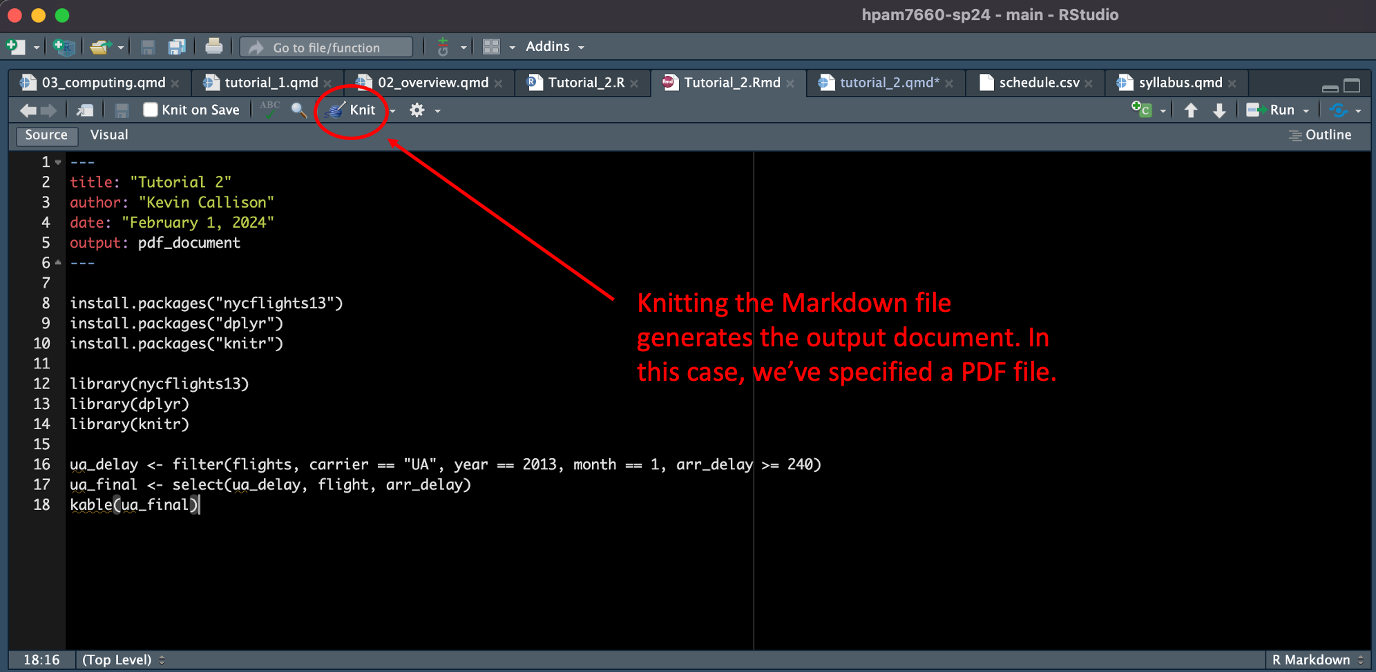
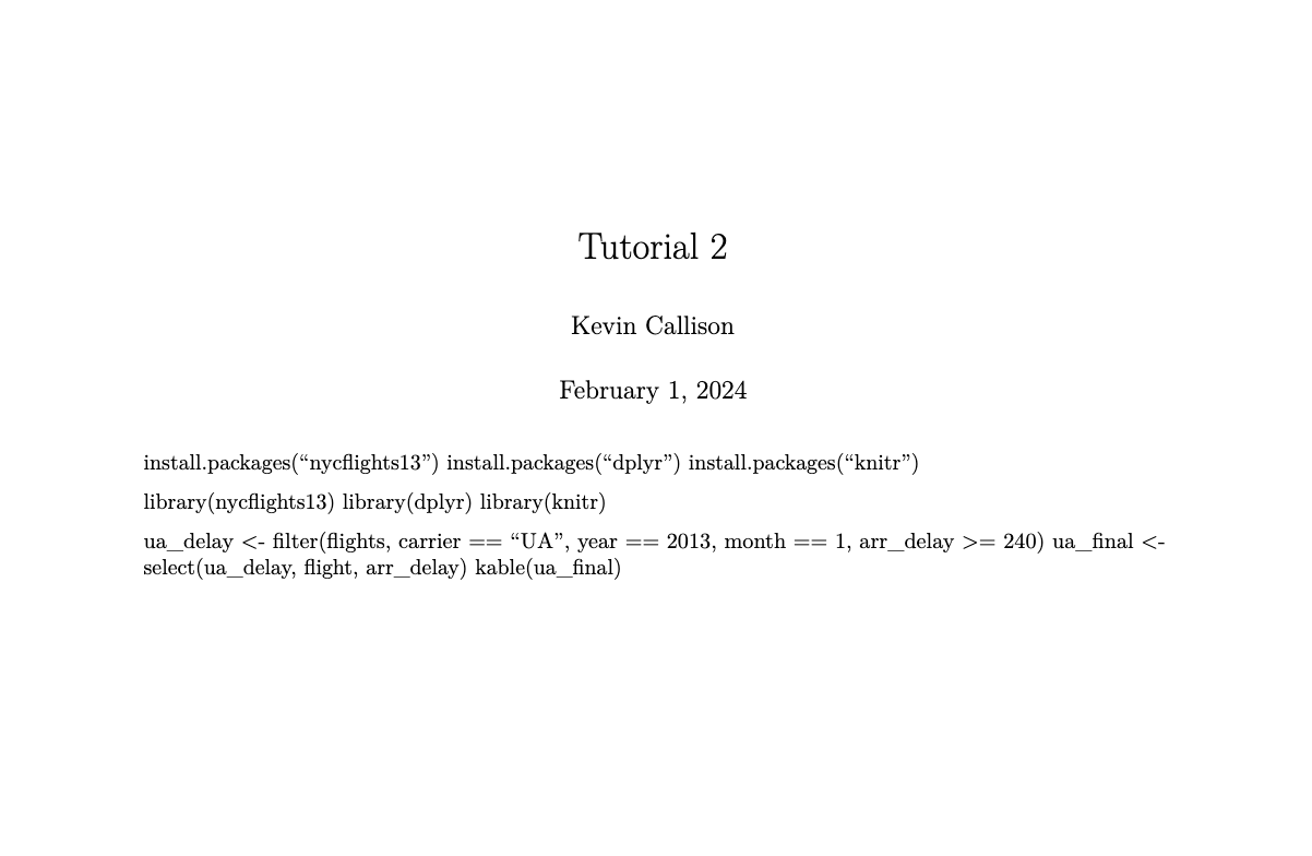
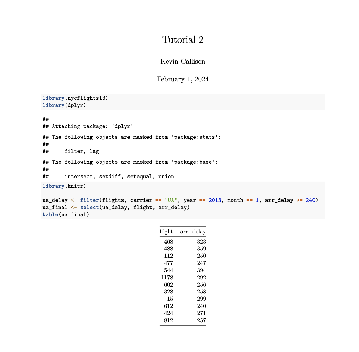
You should see a message in the “Render” tab telling you that the output has been created and now see a PDF file that includes the title, your name, the date, and the R code that you typed. Something like this:

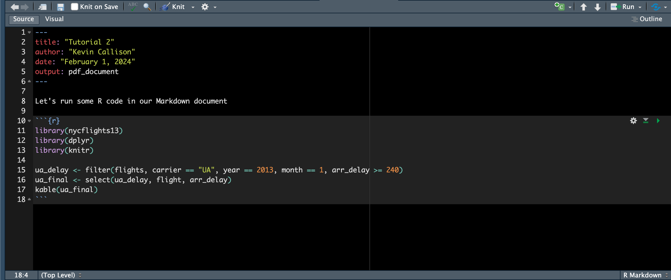
This is good, but we can do better. For one thing, Markdown doesn’t recognize the R code we included as code - it just sees it as text. But we can tell Markdown that it is R code by adding “chunk delimiters” at the beginning and end of the code. The chunk delimiters tell Markdown that this is code and not text, and knowing that, Markdown will actually run the code.

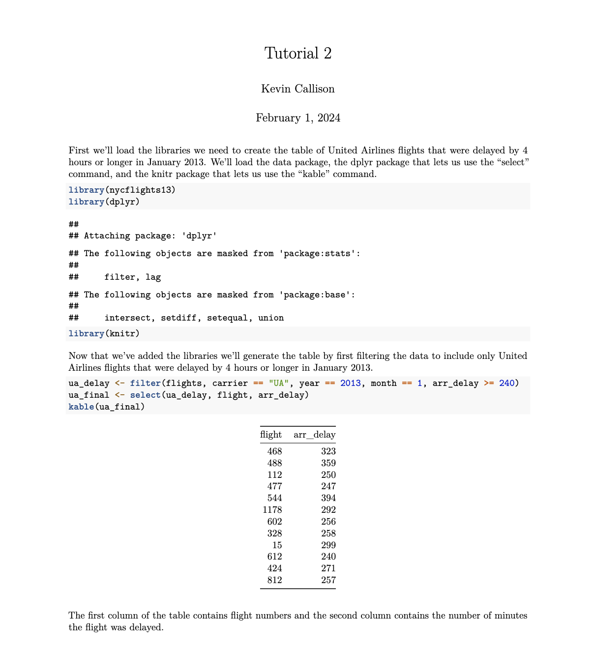
Now the PDF file contains our R code in nice grey blocks, along with any messages that R generates. More importantly, the PDF file also includes the output generated by the R commands.

It’s always good practice to annotate our code so that others know what we’re doing and why we’re doing it. Add some text to your Markdown files like I’ve done below:

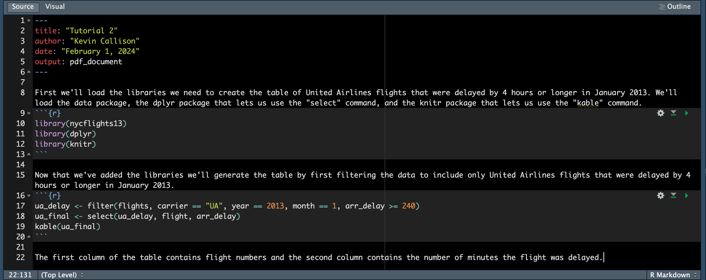
Your final result should look something like this:

Congratulations! You made it all the way through Data Lab 2!